Satellite-based edge-deployed AI

Postgraduate dissertation, University of Warwick.

Earth observation satellites can photograph far more of the planet than they can send back. They send data down in short windows while a ground station is in view, so operators spend that time on the pictures people pay for: land, and places of high economic value. Over open ocean the cameras sit idle much of the time.

That leaves some people with no way to use space at all. Most of the world's industrial fishing fleet doesn't show up in public tracking data, so the reliable way to find those boats is to look for them. A small island nation trying to catch illegal fishing across its own waters would need huge stretches of ocean imaged, and under the current model it can't pay for that. The ocean counts as low value because sending pictures of it costs more than they earn.

My MSc Applied Artificial Intelligence dissertation at WMG, supervised by Dr Mayen Cunden, goes after that cost from the satellite's end. If the spacecraft looks through its own pictures and sends home what matters, a frame of empty ocean can go down as a few coordinates instead of a full image. I used vessel detection as the test case and asked how to build image processing that runs on the satellite's own hardware, as the eyes of an AI agent that decides what to image, process and send.

The design I landed on makes the sums work for small users. One shared backbone runs on the satellite, and many tiny task-specific heads sit on top of it. The backbone is the expensive part, and it runs once for everyone. A new user's head is about 8 KB, trains in a couple of hours and fits in a single uplink window. Along the way I found that adding synthetic cloud to a small share of training images makes detectors hold up in bad weather. It took a published detector from 0.11 to 0.70 F1 on overcast frames.

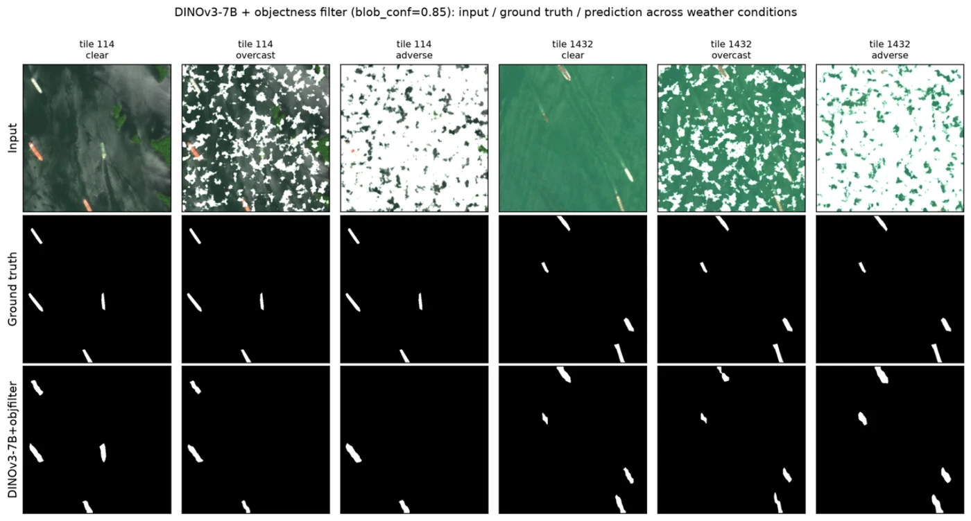
Two test scenes under clear, overcast and adverse synthetic cloud. The labels (middle) stay the same under every sky, and the DINOv3-7B pipeline (bottom) still finds most of the ships.

The problem

One estimate puts the share of recorded satellite data that reaches Earth at about 2%. I treat that figure as indicative, since it comes from a company raising money to fix what it calls the "2% problem".

I looked at whether you could raise downlink capacity instead. More ground stations help less than you'd expect, because the useful and affordable sites near well-connected cities are already saturated, and a station in the middle of the ocean would be impractical and expensive. A higher orbit gives longer contact windows but costs resolution for a given size of optics. Shannon-Hartley caps the bitrate, and the terms you can change (bandwidth, transmitter power, antenna gain) are limited by spectrum cost, the power budget and antenna design. Compression is already close to its information-theoretic limit. That leaves sending less information, which means deciding on board what is worth sending.

Vessel detection shows why this matters. Paolo et al. (2024) found that over 75% of the world's industrial fishing vessels don't appear in public AIS data, so a system built on AIS transponders can reach at most about 25% recall. Image-based detection doesn't need the ship to cooperate, but today it only runs on the small fraction of imagery that gets downlinked.

What already flies

ESA's Phi-sat-1 (2020) was the first satellite known to carry a dedicated AI payload for real-time image filtering. It ran CloudScout, a network that discarded cloudy images before downlink, on an Intel Movidius Myriad 2 drawing about 0.5 W. Phi-sat-2 (2024) added the ability to install or update models after launch. Planet's Pelican satellites carry an NVIDIA Jetson AGX Orin (a 2048-core Ampere GPU, 15 to 60 W, 64 GB of memory), and the planned Owl satellites carry a Jetson Thor with 128 GB.

These payloads run fixed inference pipelines that filter imagery for the operator. I couldn't find published work on user-defined tasks running alongside a satellite's normal operations, and operators won't give up their proven business to host one. So my requirements were a reprogrammable system that uses the high-end hardware now flying and works around the downlink limit without disrupting primary operations.

Data

The imagery came from the Planet Labs Education and Research Program: over 100,000 km² at 3 m resolution, covering open ocean and coastal water. I hand-annotated vessel masks myself and split the data 70:15:15 into training, validation and test sets, keeping frames from the same image in the same set so nothing leaked between them. Vessels cover about 0.016% of pixels, which makes for a heavy class imbalance. At 3 m you can't resolve a person, and the dataset holds no personal data.

I tested in three weather conditions: clear (under 15% cloud), overcast (15 to 50%) and adverse (over 50%). I couldn't label ships hidden under real cloud, so I built the overcast and adverse sets by adding synthetic clouds to images I'd annotated in clear conditions. That way the ground truth stays accurate however cloudy the frame looks.

Models

Chapter 3 of the dissertation is an artefact-driven narrative literature review (ART-NLR), which I used to derive requirements and candidate architectures in stages as the design needed them. It produced five model variants:

1. A CNN trained from scratch on the satellite data.
2. A pretrained ResNet, fine-tuned end to end.
3. A pretrained TIMM Vision Transformer, fine-tuned.
4. A frozen DINOv3 ViT-L backbone pretrained on satellite imagery (dinov3-vitl16-pretrain-sat493m), with a small trained head.
5. The same setup on the 7B-parameter satellite DINOv3 backbone.

DINOv3 is Meta's self-distilled model. It learns patch embeddings from unlabelled images, and you train a lightweight head on top of those embeddings for your task.

I used one model family per approach, since the goal was to find the best way to build such a system and not the single best model. All five shared the same augmentation (flips, rotation, scale jitter and colour). I tuned hyperparameters with sweeps, selected on validation IoU, and stopped training once validation loss had plateaued for 5 epochs. The sweeps took seventy-two training runs.

For a comparator I used Magalhães, Falcão and Barbosa (2025), a YOLO vessel detector on Sentinel-2 imagery that reports 90.47% precision, 86.98% recall and 88.69% F1. Their numbers come from their method on their data, so I also reproduced their configuration on my data.

How I measured it

I made instance-level detection the headline metric: whether each vessel is found at all. A ship can move kilometres between detection and interception, so a prediction a few metres off still tells the user what they need, and I didn't want to penalise that. I avoided mAP for the same reason; at 0.016% positive pixels, a close prediction with little overlap can miss an IoU threshold while still being useful. Pixel metrics (IoU, Dice, precision and recall) served as secondary measures and for tuning.

I fixed these success criteria before testing:

Criterion	Threshold	Source
Instance F1	88.7%	Magalhães, Falcão and Barbosa (2025)
Instance precision	90.5%	Same
Instance recall	87.0%	Same
Inference latency	14 ms per 512×512 tile	Keeping up with 100% of imagery at full resolution
Peak memory	64 GB	Jetson AGX Orin unified memory

The comparator reports its scores at a fixed IoU threshold and mine don't use one, so the comparison is approximate.

I didn't have flight hardware. I measured latency, power and memory on a desktop GPU with a benchmark approximating a Jetson AGX Orin, and projected latency to the Orin's 1.3 GHz clock.

Results

On validation data, the scratch CNN stayed between 0.44 and 0.49 IoU. Larger versions helped only a little, and changing the seed moved it by a similar margin. It was the model most hungry for data: 0.25 IoU on 5% of the training set, rising to 0.485 on all of it. Fine-tuned ResNet-152 reached 0.517, and fine-tuning beat freezing the backbone. Fine-tuned ViT-small matched it at 0.517, while frozen ViTs scored 0.02 to 0.16 lower than fine-tuned ones and the largest ViT overfit. Both ResNet and ViT did well on small data fractions but improved slowly as I added more. On the frozen DINOv3 backbones, the best head reached 0.483 IoU, and a single linear layer managed 0.453. Quantising the backbone to int8 or int4 changed IoU by less than 0.01.

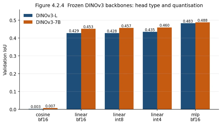
Heads on the frozen DINOv3 backbones. A linear head gets most of the way, an MLP head does best, and int8 or int4 quantisation barely moves the score.

On the clear test set at a probability threshold of 0.5, every model found most vessels (recall 0.86 to 0.95) but raised plenty of false alarms (precision 0.27 to 0.42):

Model	Instance F1 (clear test set)
DINOv3 heads (L and 7B)	0.577 and 0.574
ResNet-152	0.532
ViT-small	0.489
Scratch CNN	0.407

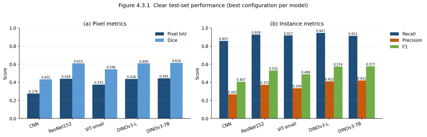
Clear test set. Every model finds most of the vessels (recall, right), and precision is what separates them.

The DINOv3 lead came from precision, which suggests their embeddings separate ships from background clutter better. Because precision was holding the 7B model back, I added an objectness filter that checks whether each predicted area is a vessel. That raised instance F1 to 0.65 and precision to 0.52, at the cost of pulling recall below the 0.87 threshold. Four of the six models in the final comparison cleared the recall bar. None came near the 0.905 precision or 0.887 F1 targets.

Across the precision-recall curves, the DINOv3 models held the highest precision at every recall level and started near 1 at low recall. The CNN sat near 0.08 precision throughout. Every curve moved inward as cloud increased, and the DINOv3 advantage was widest in adverse weather.

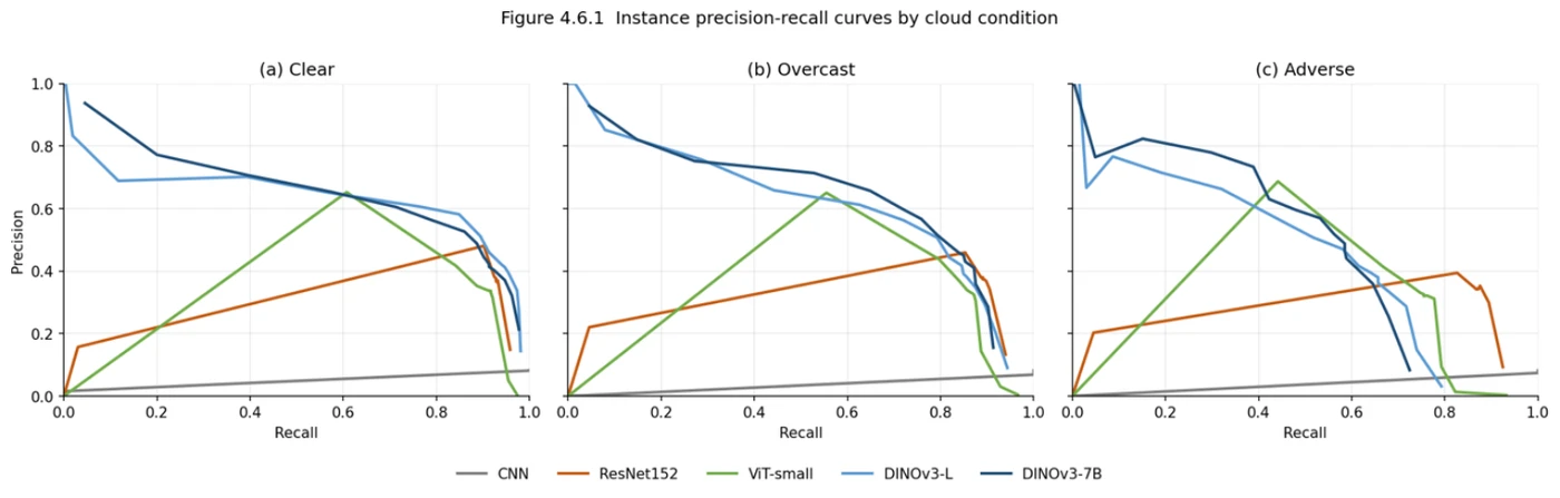
Precision against recall in each weather condition. The DINOv3 models (blues) stay on top, and the CNN (grey) sits near the floor.

Cloud augmentation gave the result I found most interesting. Adding clouds to a small share of training frames improved overcast and adverse performance with little effect on clear frames. The reproduced comparator, and my models, also did better on clear test frames after training with some clouded frames, even though they had seen fewer clear images. Pushing the share of clouded frames higher added little, with slight drops at 80% and 100%. The scratch CNN was the exception: it gained a little on cloudy frames and then got worse, and any clouded training data hurt it on clear frames.

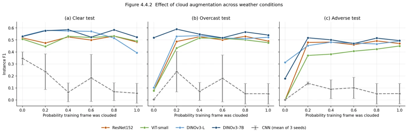
Instance F1 against the share of training frames with added cloud. Most of the gain in overcast and adverse weather arrives with the first 20%. The CNN (grey dashes, mean of three seeds) is the exception.

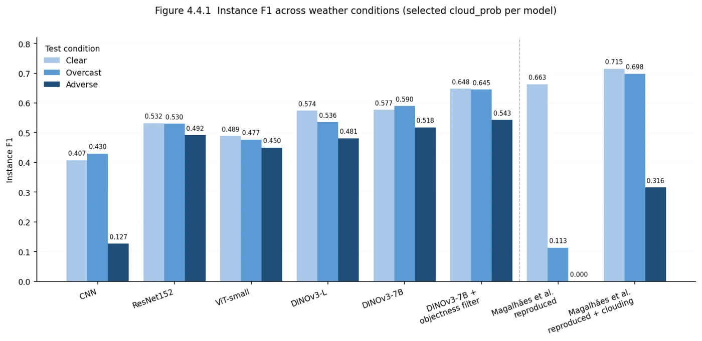
Instance F1 by weather for each model's chosen setting. The reproduced comparator scores 0.113 in overcast and 0 in adverse weather. Trained with added cloud, it reaches 0.698 and 0.316.

Resource cost at the 512-pixel operating size:

Model	Latency
Scratch CNN	15.5 ms
Reproduced comparator	43.4 ms
ViT-small	50.5 ms
DINOv3-L	95.7 ms
ResNet-152	99.5 ms
DINOv3-7B	1023 ms

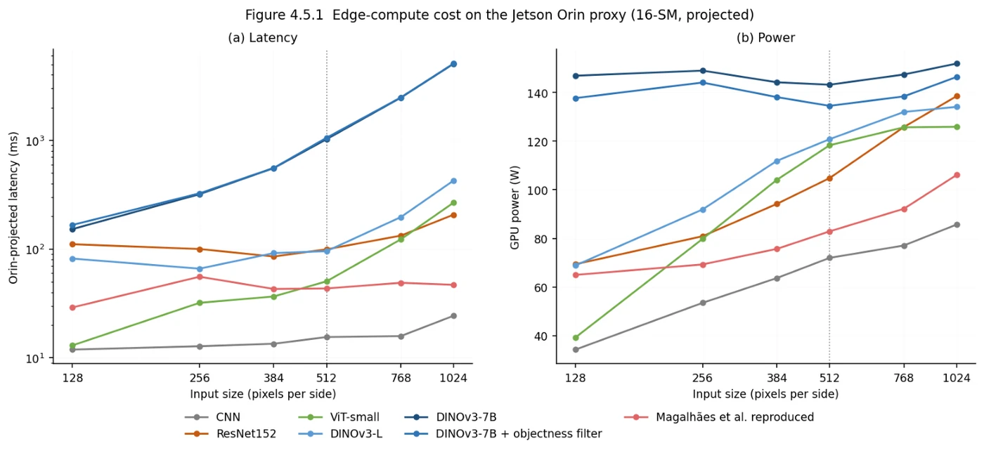
Projected latency on the Orin (left) and measured GPU power (right) as the input grows. The power figures come from a desktop card at boost clock, so compare them with each other and not with flight hardware.

The objectness filter added 2.9 ms to the 7B pipeline. Peak memory ran from 0.02 GB for the CNN to 12.6 GB for the 7B (0.15 GB for the comparator), all inside the 64 GB budget. No model got under 14 ms, so a real deployment would need to process a fraction of the imagery or downscaled frames. GPU power ran from 72 W to 143 W, but I measured it at the desktop card's boost clock, so it says little about power draw on flight hardware. The 7B backbone gave a negligible gain over DINOv3-L while running about ten times slower.

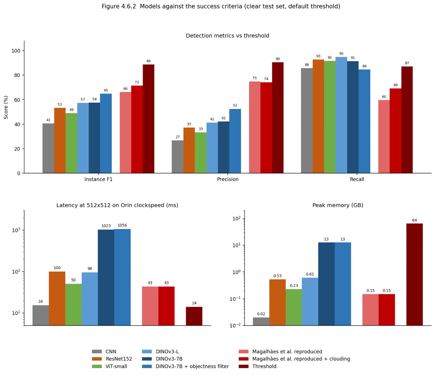
Every model against the success criteria, shown in dark red. Recall clears the bar for most models; precision, F1 and latency don't.

The shared backbone

The answer I reached is to run one quantised, self-distilled backbone trained on satellite imagery, and let many small user-defined heads read its patch embeddings. The satellite then downlinks the heads' outputs, or acts on them.

The argument is mostly about cost. The backbone takes over 1000 ms and up to 12.6 GB, while a head takes about 2 to 3 ms and 8 KB to 1 MB of memory. You could run hundreds of heads before they cost as much as the backbone, so each new customer adds very little. Uplink points the same way. A trained head is about 8 KB and fits in one contact window, while a ResNet-152 U-Net is about 196 MB, roughly 51 minutes of continuous uplink at 512 kb/s. The backbone only goes up once, possibly before launch, and quantisation to int8 or int4 shrinks it with almost no loss. Training a head takes a couple of hours on modest hardware, which one ML engineer can handle without a model development team.

I didn't set this out as a success criterion at the start. It's the main reason I'd pick DINOv3.

Where the agent comes in

What I built is the perception layer for an agent. It doesn't make decisions itself. A satellite spends resources imaging, processing and transmitting, and an agent could skip any of those steps: not imaging at night or where no one wants data, not processing a frame that's heavily clouded or already booked for downlink, and choosing between sending detections, small crops of likely vessels or a whole image. Building that part needs access to spacecraft hardware, or a deep knowledge of how its systems work, and was out of scope.

Limitations

• The clouds are synthetic. They let me keep accurate labels, but they imitate real cloud.
• I labelled every image myself, so one person's errors run through the whole dataset.
• All the imagery came from one provider.
• I tested one model family per architecture, and other families might change the conclusion.
• I reported headline figures at a 0.5 probability threshold. A real user's requirements might favour a different one.
• The hardware numbers come from a desktop proxy. Flight hardware adds competing programmes, heat and power limits, radiation-induced bit flips and the operator's own safeguards against crashes.

I also couldn't find published end-user requirements for detection confidence, acceptable latency or operating thresholds, which is why I borrowed the success criteria from a comparator paper.

Further work

Anyone continuing this should start by establishing those end-user requirements. After that, I'd like to see a backbone whose embeddings ignore cloud, possibly trained with the clouding technique used here. I'd also like to try federated training of the backbone on board the spacecraft, which would let it learn from every image the satellite takes, including the ones that never get downlinked.