I want snow on my birthday

I found out a while ago that the UK is more likely to get snow at Easter than at Christmas. My birthday falls at the start of April, close to Easter, and I've never seen snow anywhere near it.

I knew about climate change, and I'd heard the 1.5°C warming figure plenty of times, but I didn't understand what 1.5°C meant for the weather on an actual day. I wanted to be able to look at a date and say, oh wow, that's what my birthday is supposed to feel like.

You pick a city and a date, and the page gives you the day of the year that now has the temperature your birthday had before industrialisation. It compares temperatures and nothing else, so it can't promise you snow.

For a given city I build two smooth curves of daily mean temperature through the year, one for a pre-industrial climate and one for the present day. Your birthday sits on the old curve at some temperature. I look along the new curve for the day that now has that temperature, and that day is your climate birthday. In most places the answer is earlier in spring and later in autumn, because the whole curve has moved up.

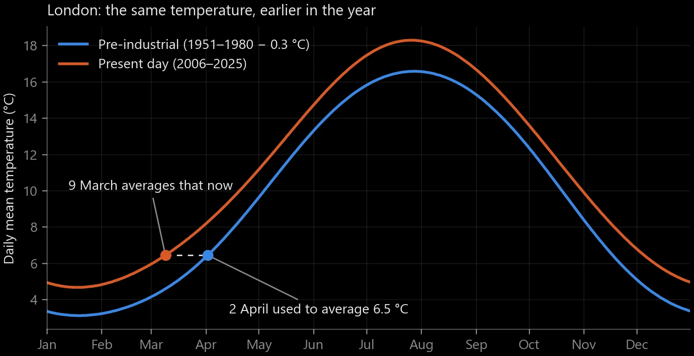
London's two curves. 2 April used to average 6.5 °C, and the present-day curve reaches 6.5 °C on 9 March, 24 days earlier.

The code is on GitHub at JacobRhys/climate-birthday if you want to check any of the steps below against it.

The statistical analysis

Step 1: the data

Cities

I don't geocode anything. The CITIES list in build.py holds 93 places I typed in by hand, each with an id, a name, a country and a latitude and longitude to three decimal places. The list runs from Longyearbyen at 78.2° N to the South Pole, which I entered as $-89.98^\circ$ latitude.

Download

fetch_daily sends each city's coordinates to the Open-Meteo archive API and asks for one variable, temperature_2m_mean: the daily mean air temperature 2 metres above the ground. It also sets timezone=auto, so a "day" is the local calendar day at that city and not a UTC day.

I don't pick or interpolate grid cells myself. I don't pass a models parameter either, so the API uses its default "best match", which stitches three ECMWF datasets together: ERA5 ($0.25^\circ$, about 28 km, 1940 onwards), ERA5-Land ($0.1^\circ$, about 11 km, 1950 onwards) and the IFS HRES forecast model (9 km, 2017 onwards). Over land it looks for a nearby cell with a similar elevation to the requested point, using a 90 m elevation model, and then adjusts the temperature statistically for the difference in height.

The daily mean is Open-Meteo's, not mine. It averages the 24 hourly values of the local day:

$$ T_j = \frac{1}{24} \sum_{h=0}^{23} T_{j,h}, $$

where $T_{j,h}$ is the 2 m temperature in hour $h$ of day $j$.

The API returns degrees Celsius by default, and the code never converts units. Every temperature in this post, in cities.json and on the page is in °C. Days with no value come back as null, and fetch_daily turns them into NaN so a later step can drop them.

For one city and one period, the result is a list of pairs $(t_j, T_j)$, where $t_j$ is a calendar date and $T_j$ is that day's mean 2 m temperature in °C.

build_city makes two requests per city, one per period, because long daily requests count heavily against the free quota and trigger HTTP 429 errors. fetch_daily caches every raw response in data/climate_birthday/cache/, keyed by latitude, longitude, start and end date, so a rerun downloads nothing it already has. On a 429 it waits 60 s and tries once more. Any other HTTP error stops it straight away. Network errors get up to six attempts, with waits of 5, 10, 15, 20 and 25 s between them. If a city still hits an HTTP error, main skips it, writes the cities it did get, and exits with an error listing the missing ones.

Step 2: the two periods

The periods are constants at the top of build.py:

$$ P_{\text{base}} = [1951,\ 1980], \qquad P_{\text{cur}} = [2006,\ 2025] $$

The baseline request covers 1 January 1951 to 31 December 1980. The current request covers 1 January 2006 to 31 December 2025, or to the day of the build if that comes first. I ran the build after 2025 ended, so both periods are complete: 30 years for the baseline and 20 for the present. At that length a single hot or cold year moves the curve very little.

I wanted 1850 to 1900 for the baseline, the usual definition of pre-industrial, but ERA5 starts in 1940. I left the 1940s out as well. ERA5's back extension before 1950 rests on sparse observations and runs warm in several regions; Delhi's 1940s sit 0.7 °C above its 1950s. So I use 1951 to 1980, the standard GISS reference period, and later subtract a fixed offset to stand in for the older climate (Step 4).

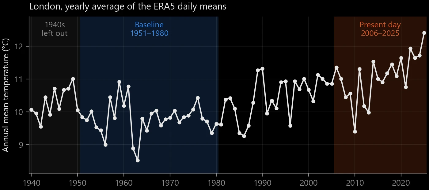
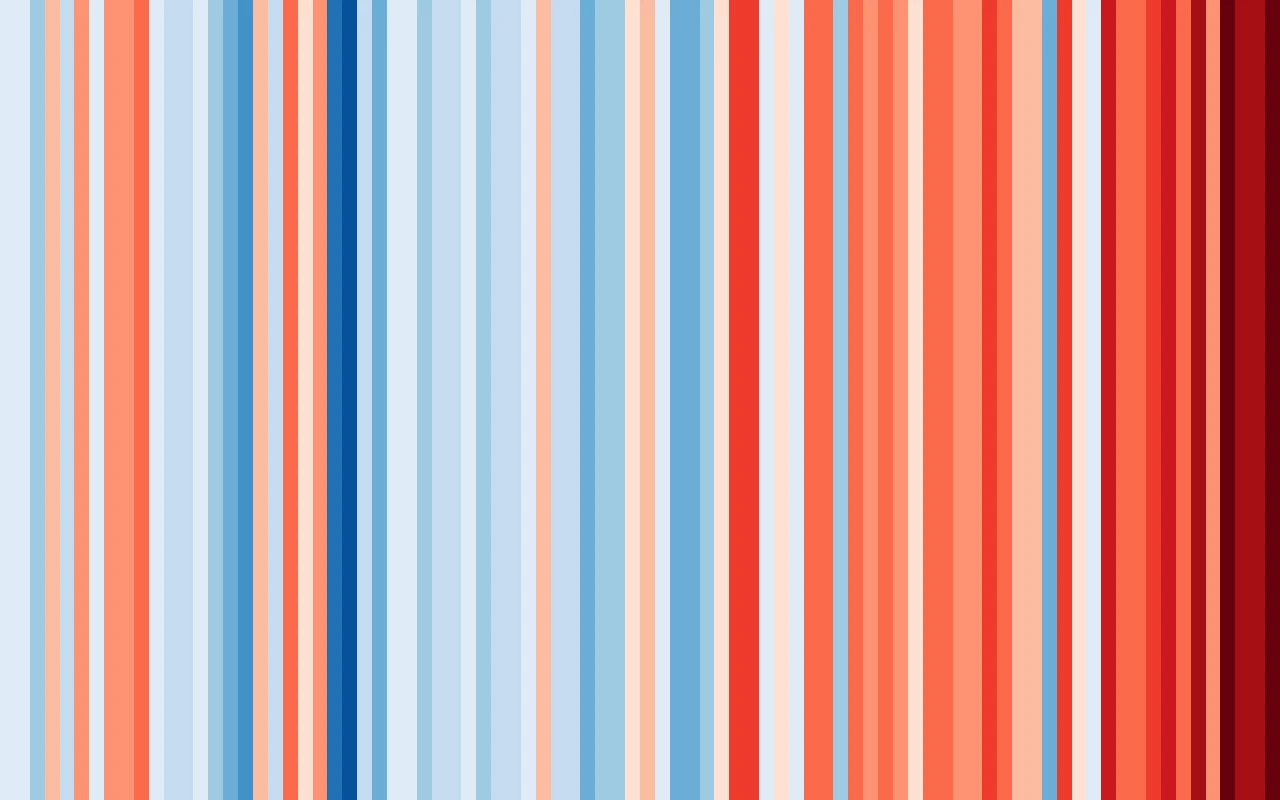
London's yearly mean from the same Open-Meteo data, with the two periods shaded. The stripes at the top of this post show the same yearly means as colours.

Inside climatology, the code keeps the samples that fall in the period and have a value:

$$ \mathcal{J}_P = \{\, j : y_0 \le \operatorname{year}(t_j) \le y_1,\ T_j \ne \mathrm{NaN} \,\} $$

where $[y_0, y_1]$ is the period $P$ and $\mathcal{J}_P$ is the set of indices of the samples that go into the fit.

Precision against accuracy

Picking the baseline years trades one kind of error for another. Precision is how much the answer would move if the same years had brought different weather. Accuracy is how close the answer sits to what I want to compare against, the climate before industrialisation.

A recent baseline buys precision. ERA5 has far more observations to work from after 1950, and 30 years is enough to average out single odd years. London's yearly averages over 1951 to 1980 have a standard deviation of 0.50 °C, so the 30-year mean carries a standard error of about 0.09 °C. The 20-year present-day window is looser, at 0.16 °C.

The cost is accuracy. Every decade after 1900 has some warming in it, and the later the baseline starts, the more warming I have to take back out with an offset. That offset is a global figure standing in for a local one. London's 1981 to 2010 mean sits 0.66 °C above its 1951 to 1980 mean, so a baseline that late would need that much more removed on top of the 0.3 °C, and any error in the offset goes into the answer.

An older baseline swaps the problem round. It sits closer to pre-industrial and needs a smaller offset, but the reanalysis has less to go on and its errors grow. London shows the risk: its ERA5 1940s average 10.31 °C, 0.51 °C above 1951 to 1980. A decade closer to pre-industrial coming out warmer is a warning sign, the same one Delhi gives.

For a birthday, the error turns into days. Where London's present-day curve crosses 2 April's old temperature, it climbs 0.07 °C a day, so every 0.1 °C of error in the baseline moves the climate birthday by about 1.4 days. Dropping the $-0.3$ °C offset would move London's answer from 9 March to 13 March, and doubling it would give 4 March. With 1951 to 1980, I get 30 well-observed years, and an offset small enough that a 0.1 °C mistake costs London about a day and a half.

Step 3: day of year and leap days

The fit needs every sample placed on a 365-day year. day_of_year takes each date's 0-based ordinal $n_j$ (1 January is $n_j = 0$) and folds 29 February onto 28 February:

$$ d_j = \min\!\big(364,\ \max(0,\ n_j - \ell_j)\big), \qquad \ell_j = \begin{cases} 1 & \text{if } \operatorname{year}(t_j) \bmod 4 = 0 \text{ and } n_j \ge 59,\\ 0 & \text{otherwise.} \end{cases} $$

In a leap year $n_j = 59$ is 29 February. Subtracting one puts it on slot 58, which is 28 February, and moves 1 March onwards back by one day so every date after February lands on the same slot it would have in a normal year. The cost is that 28 February gets two samples in each leap year instead of one. The divisible-by-four test gets century years wrong, but no century year falls in either period, so it gives the right answer for this data. The clip to $[0, 364]$ never triggers after the fold; it is a guard.

Step 4: fitting the seasonal cycle

The matching in Step 6 inverts the present-day curve: it looks for every day where the curve crosses a given temperature. A raw day-of-year average still carries weather noise, and a noisy curve crosses a given temperature many times. I replace each period's data with a smooth curve made of a few sine waves.

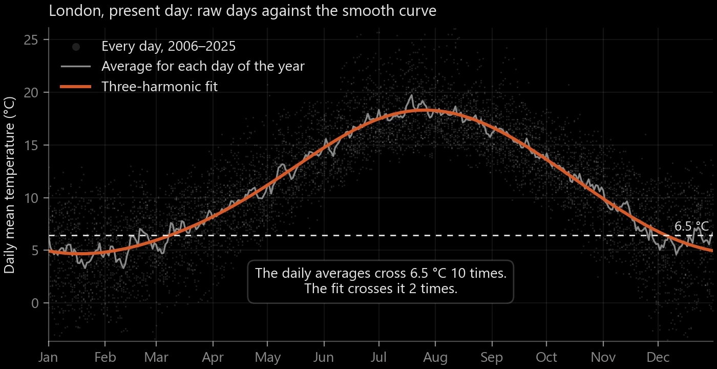
Every London day from 2006 to 2025, the average for each day of the year, and the fitted curve. At 6.5 °C, 2 April's old temperature, the daily averages cross 10 times and the fit crosses twice.

The model

climatology turns each day slot into an angle around the year,

$$ \theta_j = \frac{2\pi d_j}{365}, $$

and fits a Fourier series with $K$ harmonics:

$$ f(\theta) = a_0 + \sum_{k=1}^{K} \big( a_k \cos k\theta + b_k \sin k\theta \big), \qquad K = 3. $$

$K$ is the constant HARMONICS. The $k = 1$ term is the annual cycle, and $k = 2, 3$ are the two overtones that let spring and autumn differ in shape (a slow spring and a fast autumn, say). The model has $2K + 1 = 7$ coefficients: $a_0$ is the annual mean and $a_k$, $b_k$ set the size and timing of each harmonic.

Least squares on the raw days

I don't average by day of year first. climatology fits the model to every daily sample at once, with np.linalg.lstsq:

$$ \hat{\boldsymbol\beta} = \arg\min_{\boldsymbol\beta} \sum_{j \in \mathcal{J}_P} \big( T_j - f(\theta_j;\ \boldsymbol\beta) \big)^2, \qquad \boldsymbol\beta = (a_0, a_1, b_1, a_2, b_2, a_3, b_3). $$

In matrix form each sample is one row of a design matrix $X$:

$$ X_{j,\cdot} = \big(1,\ \cos\theta_j,\ \sin\theta_j,\ \cos 2\theta_j,\ \sin 2\theta_j,\ \cos 3\theta_j,\ \sin 3\theta_j\big), \qquad \hat{\boldsymbol\beta} = \arg\min_{\boldsymbol\beta} \lVert X\boldsymbol\beta - \mathbf{T} \rVert_2^2 . $$

With no gaps, the baseline has $30 \times 365 + 8 = 10{,}958$ rows (eight leap days, 1952 to 1980) and the present day has $20 \times 365 + 5 = 7{,}305$ rows. Every slot gets 30 or 20 samples apart from 28 February, so this fit comes out close to a fit on the 365 day-of-year means. The differences come from missing values and the doubled 28 February.

From coefficients to 365 numbers

climatology then evaluates the fitted curve at the 365 day slots, and build_city adds the pre-industrial offset to the baseline only:

$$ B_d = \hat f_{\text{base}}\!\left(\frac{2\pi d}{365}\right) + \Delta, \qquad C_d = \hat f_{\text{cur}}\!\left(\frac{2\pi d}{365}\right), \qquad d = 0, 1, \dots, 364, $$

with

$$ \Delta = -0.3\ ^\circ\mathrm{C}. $$

$B_d$ is the pre-industrial temperature on day slot $d$ and $C_d$ is the present-day one. $\Delta$ is the constant PREINDUSTRIAL_SHIFT_C, the approximate global mean warming between 1850-1900 and 1951-1980. The same 0.3 °C goes to every day of every city. Local warming over that stretch varied from place to place, so this offset is the weakest part of the method. A daily per-city series from Berkeley Earth, which goes back to 1880, would replace it with the same output format.

Last, build_city rounds both curves to two decimal places before writing them to cities.json:

$$ B_d \leftarrow \frac{\operatorname{round}(100\,B_d)}{100}, \qquad C_d \leftarrow \frac{\operatorname{round}(100\,C_d)}{100}. $$

Everything from here on runs in the browser on these rounded values.

What three harmonics buy

$f(\theta) - T$ is a trigonometric polynomial of degree 3, and a polynomial like that has at most $2K = 6$ roots per period. So the smooth present-day curve can cross any temperature at most six times a year, and in a typical mid-latitude city it crosses twice, once on the way up and once on the way down. The fit does not force the curve to be monotonic between its coldest and warmest days; the comment in build.py hopes for that shape but nothing enforces it. Step 6 copes with extra crossings when they occur. The price of the smoothing is that three harmonics cannot hold a sharp seasonal feature such as the onset of a monsoon.

Step 5: turning your birthday into a day slot

You pick a day and a month. App.tsx clamps the day to the month's length on a 365-day calendar (so 29 February becomes 28 February, the same fold as Step 3), and toDoy converts it to a 0-based slot:

$$ d_0 = \sum_{m=1}^{M-1} L_m + \min(D,\ L_M) - 1, \qquad L = (31, 28, 31, 30, 31, 30, 31, 31, 30, 31, 30, 31), $$

where $M$ is the month (1 to 12), $D$ is the day of the month and $L_m$ is the length of month $m$. For 2 April, $d_0 = 31 + 28 + 31 + 2 - 1 = 91$.

Step 6: finding the climate birthday

climateBirthday in mapping.ts does the matching. It starts by reading the pre-industrial temperature on your birthday:

$$ T^{\ast} = B_{d_0}. $$

Which half of the year you're in

A spring temperature also turns up in autumn, and I want 2 April to map to another spring day, not to October. slopeSign records whether the old curve was rising or falling on your birthday, with a central difference:

$$ p = \operatorname{sgn}\!\big( B_{[d_0 + 1]} - B_{[d_0 - 1]} \big), \qquad [i] = i \bmod 365 . $$

The brackets are the wrap helper, which lets 1 January look back to 31 December. $p = +1$ means warming season, $p = -1$ cooling season, and $p = 0$ means the birthday sits on a turning point. The test uses the slope and not the calendar, so it works in the southern hemisphere without any special case.

Every crossing of the present-day curve

crossings walks the 365 segments of the present-day curve. Segment $i$ joins $C_i$ to $C_{[i+1]}$, so segment 364 joins 31 December to 1 January and a crossing over New Year still counts. For each segment:

$$ \text{if } C_i = T^{\ast}: \quad x = i, \quad s = \operatorname{sgn}\!\big( C_{[i+1]} - C_{[i-1]} \big); $$

$$ \text{else if } T^{\ast} \text{ lies strictly between } C_i \text{ and } C_{[i+1]}: \quad \tau = \frac{T^{\ast} - C_i}{C_{[i+1]} - C_i}, \quad x = i + \tau, \quad s = \operatorname{sgn}\!\big( C_{[i+1]} - C_i \big). $$

$x$ is a fractional day slot where the straight line between the two daily values reaches $T^{\ast}$, $\tau \in (0, 1)$ is how far along the segment that happens, and $s$ is the direction the present-day curve is moving there. A crossing that lands on a segment's far end is not counted in that segment; it is counted by the next one, where it is the near end, so no crossing appears twice. A crossing on the New Year segment has $x$ between 364 and 365.

Picking one

The code keeps the crossings that move in the same direction as your birthday did:

$$ \mathcal{X}_p = \begin{cases} \{\, x : s = p \,\} & \text{if } p \ne 0,\\ \text{all crossings} & \text{if } p = 0. \end{cases} $$

If $\mathcal{X}_p$ is empty, the code falls back to all crossings and sets phaseFallback, and the page adds a note that it found no same-season match and is showing one from the opposite season. From the remaining pool it takes the crossing nearest your birthday around the circle of the year. circularDelta gives the signed distance

$$ \delta(a, b) = b - a + 365\,k, \qquad k \in \mathbb{Z} \text{ chosen so that } \delta(a, b) \in (-182.5,\ 182.5], $$

and the climate birthday is

$$ d^{\ast} = \arg\min_{x \in \mathcal{X}_p} \big| \delta(d_0, x) \big| . $$

The loop only replaces its current best on a strictly smaller distance, so if two crossings tie, the one found first in the scan from 1 January wins. The same rule settles any extra crossings a wobbly curve might produce: the nearest same-direction one wins.

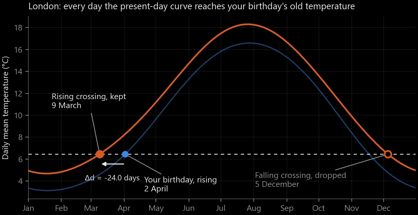
For London and 2 April, the present-day curve reaches 6.5 °C twice. The phase rule drops the falling crossing on 5 December and keeps the rising one on 9 March.

The shift and the warming

The shift and the warming on the day itself are

$$ \Delta d = \delta(d_0, d^{\ast}), \qquad w = C_{d_0} - B_{d_0}, $$

with $\Delta d$ in days (negative means earlier in the year) and $w$ in °C. For London and 2 April, $\Delta d = -24$ days.

If $w < 0$, the data has that date cooler today than in 1951-1980 even after the $-0.3$ °C offset. That happens in parts of South Asia, where irrigation and aerosols have cooled the surface.

Step 7: days whose weather no longer exists

Before looking for crossings, climateBirthday checks whether any exist:

$$ \text{extinct} = \begin{cases} \text{cold} & \text{if } T^{\ast} < \min_d C_d,\\ \text{hot} & \text{if } T^{\ast} > \max_d C_d,\\ \text{none} & \text{otherwise.} \end{cases} $$

If your birthday's old temperature is below the coldest day of the present-day year, no day is left for it to move to, and that weather has gone from the city's calendar. The hot case is the mirror image and rare. When the check says "none", the present-day curve is a closed loop that reaches both below and above $T^{\ast}$, so the scan in Step 6 finds at least one crossing.

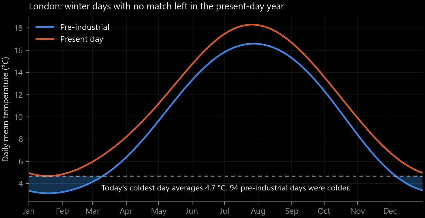
In London, 94 days of the pre-industrial winter averaged colder than today's coldest day at 4.7 °C. A birthday on any of them has no day left to move to.

The reverse question is whether today's weather on your birthday used to happen at all:

$$ \text{novel} = \begin{cases} \text{hot} & \text{if } C_{d_0} > \max_d B_d,\\ \text{cold} & \text{if } C_{d_0} < \min_d B_d,\\ \text{none} & \text{otherwise.} \end{cases} $$

A hot result means your birthday is now warmer than the warmest day of the pre-industrial year, so that weather never used to happen there.

Counting over the whole year

yearSummary runs the same tests on all 365 days:

$$ N_{\text{gone}} = \#\{\, d : B_d < \min_{d'} C_{d'} \ \text{or}\ B_d > \max_{d'} C_{d'} \,\}, $$

$$ N_{\text{new}} = \#\{\, d : C_d > \max_{d'} B_{d'} \ \text{or}\ C_d < \min_{d'} B_{d'} \,\}, $$

$$ \bar w = \frac{1}{365} \sum_{d=0}^{364} \big( C_d - B_d \big). $$

$\#$ counts the days that meet the condition, and $\bar w$ is the mean warming in °C. The mean has a short form. Each harmonic $\cos(2\pi k d/365)$ or $\sin(2\pi k d/365)$ with $k = 1, 2, 3$ sums to zero over the 365 slots, so apart from the two-decimal rounding,

$$ \bar w = \hat a_0^{\,\text{cur}} - \big( \hat a_0^{\,\text{base}} + \Delta \big) = \hat a_0^{\,\text{cur}} - \hat a_0^{\,\text{base}} + 0.3\ ^\circ\mathrm{C}. $$

The 0.3 °C offset feeds straight into all three numbers. Lowering the baseline by 0.3 °C pushes more baseline days below the present-day minimum, so it raises $N_{\text{gone}}$ as well as $\bar w$.

A worked example

The numbers in this section are made up to show the arithmetic. They don't come from any real city.

Say your birthday is 2 April, so $d_0 = 91$, and a city's baseline curve has $B_{90} = 8.21$, $B_{91} = 8.40$ and $B_{92} = 8.59$. The target is $T^{\ast} = 8.40$ °C and the slope sign is $p = \operatorname{sgn}(8.59 - 8.21) = +1$, so the birthday is in the warming half of the year.

Suppose the present-day curve has its coldest day at 4.9 °C, so $T^{\ast}$ is above $\min_d C_d$ and the weather still exists. Scanning $C$ finds two crossings of 8.40 °C. One is in autumn, on a falling segment, so $s = -1$ and the phase rule drops it. The other is on the segment with $C_{75} = 8.28$ and $C_{76} = 8.46$:

$$ \tau = \frac{8.40 - 8.28}{8.46 - 8.28} = \frac{0.12}{0.18} \approx 0.667, \qquad x = 75.667, \qquad s = +1 . $$

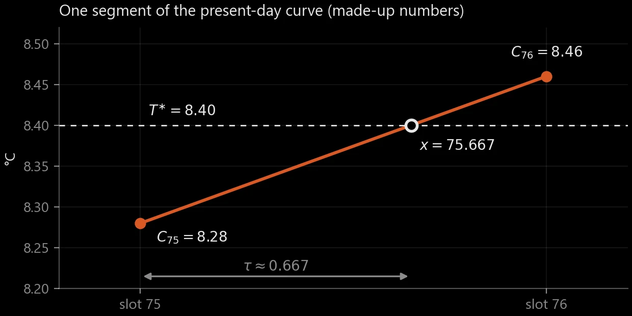
The rising segment from this example. The crossing sits two thirds of the way from slot 75 to slot 76.

That is the only same-direction crossing, so $d^{\ast} = 75.667$. The shift is $\Delta d = 75.667 - 91 = -15.33$ days, and rounding $d^{\ast}$ gives slot 76, which is 18 March. If $C_{91} = 9.55$, the warming on 2 April itself is $w = 9.55 - 8.40 = 1.15$ °C. The page would say that in this city 18 March now feels like 2 April used to, 15 days earlier.

Displaying the statistics

This part runs in App.tsx, Globe.tsx and Chart.tsx. The page loads cities.json once and reruns climateBirthday for all 93 cities each time you change the date, so every label on the globe updates at once.

Picking a birthday

The page opens on a picker set to today's date. The day list follows the month you choose on a 365-day calendar, so February stops at 28, and toDoy turns your choice into the slot $d_0$ from Step 5.

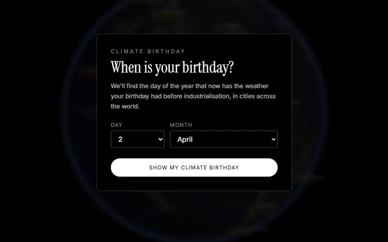
The picker, set to 2 April.

The globe

Globe.tsx draws a three.js Earth with a label on each city: its name, and under it the climate birthday as a short date, or "gone" when the birthday's weather is extinct (Step 7). The dot's colour shows how far the date moved in either direction. It blends from green at 0 days through yellow at 15 to red-orange at 30 or more, and extinct cities get a flashing red dot.

Cities on the far side of the globe, or close to its edge, are hidden. Where labels crowd together, the globe places them in order: the selected city first, then the ones that face you most. A label that lands within 96 by 30 pixels of one already placed keeps its dot and hides its text until you hover over it or zoom in. Clicking a city turns the globe to face it and draws a line from its dot to the readout card.

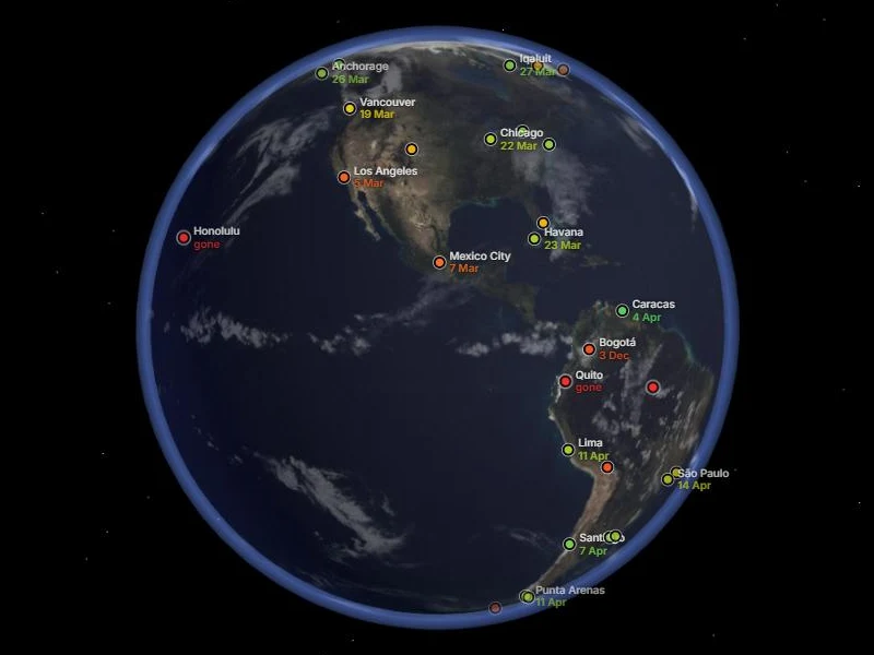
2 April over the Americas. Honolulu and Quito have no match left, and Mexico City's birthday weather now arrives on 7 March.

The readout card

The card's headline reads "In [city], the [climate birthday] now feels like the [birthday] used to", with the matched date in its dot's colour. fromDoy rounds $d^{\ast}$ to the nearest slot, $[\operatorname{round}(d^{\ast})]$, so 364.6 becomes 1 January. The sentence under the headline gives $|\operatorname{round}(\Delta d)|$ days and says "earlier" when $\Delta d < 0$ and "later" otherwise, so a zero shift reads as "0 days later". It also gives the old and new temperature on your birthday and $w$ with its sign.

A few results change the card. An extinct birthday gets a headline saying its weather no longer happens in that city, with $T^{\ast}$ next to today's coldest (or hottest) day. A novel result adds a line saying today's birthday is hotter (or colder) than any day of the pre-industrial year there. When no same-direction crossing exists, the card says it is showing the nearest match from the opposite season. When $w < 0$, a small note asks you to treat the readout with caution.

The chart

Chart.tsx draws both curves as an SVG across the year, pre-industrial in blue and present day in orange. A dashed line marks $T^{\ast}$, and a white arrow runs along it from your birthday to your climate birthday. Moving the pointer over the chart shows a crosshair and both temperatures for that day. The temperature axis rounds out to the nearest 5 °C and adds 2 °C of room at each end.

The three tiles

Under the chart, three tiles show the whole-year numbers from Step 7 for the selected city: "Avg warming" is $\bar w$, "Days gone" is $N_{\text{gone}}$ and "Days new" is $N_{\text{new}}$. They describe the city, so they stay the same whatever birthday you pick.

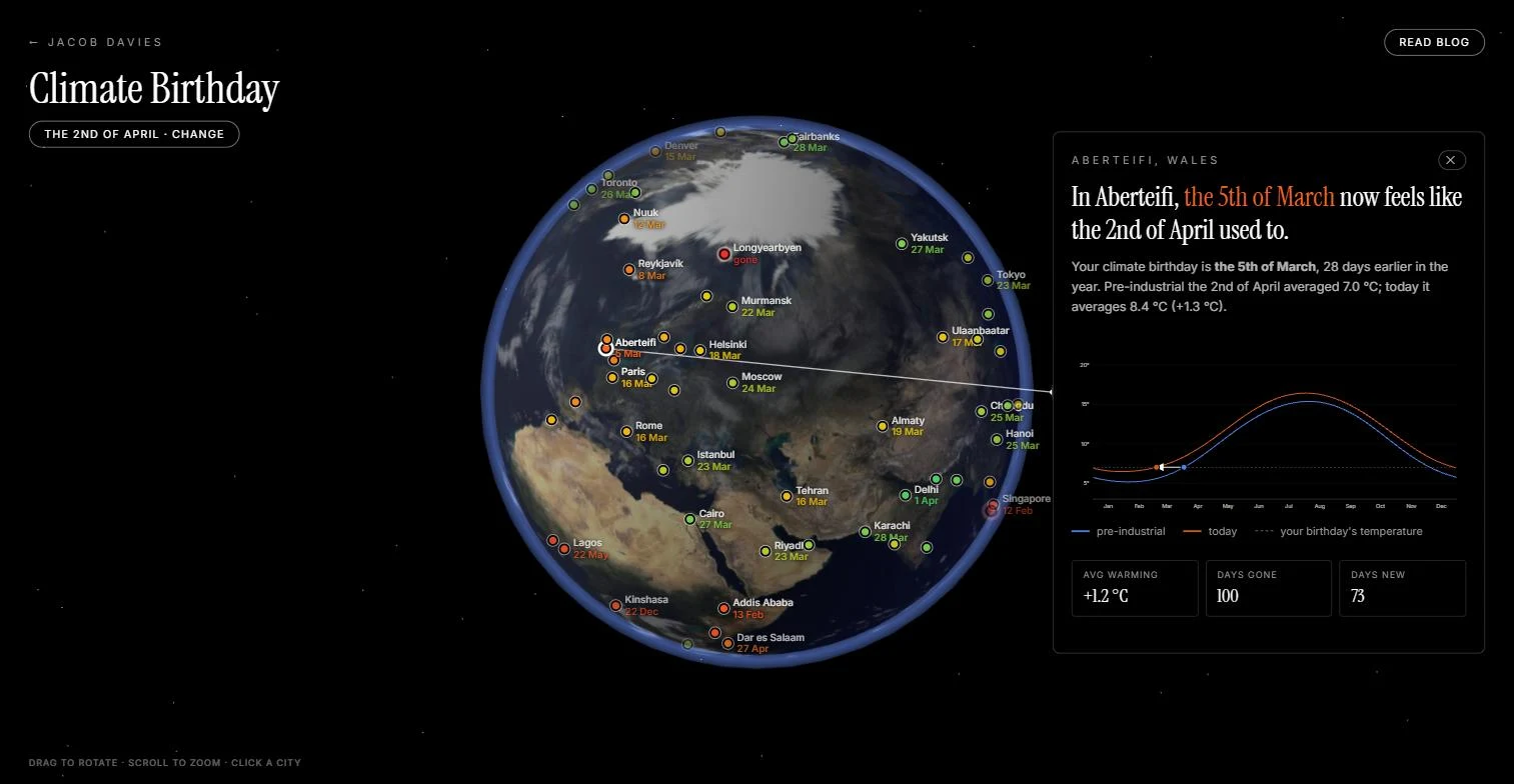
The card for Aberteifi on 2 April: 5 March, 28 days earlier. London's dot sits under Aberteifi's with its text hidden by the crowding rule.

Limitations

• Each city is one grid cell, 11 to 28 km across depending on the dataset, picked and height-adjusted by Open-Meteo. A cell that mixes sea and land or sits on steep ground (Cape Town, La Paz, Quito) can differ from what a thermometer in the city records.
• The two periods don't come from quite the same data. Open-Meteo's default blend brings in IFS HRES from 2017, so the last nine years of the present-day period partly come from a forecast model that the 1951-1980 baseline never uses. Asking for models=era5 in both requests would keep them consistent, at the cost of the coarser grid.
• The pre-industrial curve is 1951-1980 minus a flat 0.3 °C. That is a global average applied everywhere; the Arctic warmed faster than that before 1950, and other places warmed less.
• The method only uses daily mean temperature. Two days with the same mean can differ in humidity, rain and daily range, and none of that enters the match.
• Three harmonics smooth away short, sharp seasonal features.
• Where the seasonal cycle is flat, as in Singapore or Quito, a fraction of a degree of warming moves the matched date by weeks, and a large share of the old year can come out as extinct. The arithmetic is right, but the date shift says more about how flat the curve is than about how much the climate has changed.

Try it on the interactive globe below.