Writing the missing manual for AI weather forecasts

Undergraduate dissertation, University of Birmingham.

Weather forecasts save lives. Between 2000 and 2019, about 5 million people a year died from extreme temperatures alone, and every warning that gets people out of harm's way depends on a forecast that arrives in time and turns out right. Forecasts have come a long way in the last 75 years, but the traditional route has hit a wall: more data, better hardware and far bigger compute budgets now buy only small gains. Medium-range forecasts, 3 to 10 days ahead, feel this most. They need a model of the whole globe, and even the best of them struggle past about 7 days.

Machine learning weather prediction (MLWP) broke through that wall. Until late 2022 the pessimistic view was that it would not be viable before the early 2030s. Then Huawei's Pangu-Weather matched a modern numerical model while using 99.999% less computing power, and Google has since built models that beat the physics-based systems. MLWP looks like the future of medium-range forecasting.

The national weather services were left standing. When I wrote the dissertation, the Met Office, ECMWF and NOAA had nothing remotely comparable of their own, despite the money at stake. What held them back was information. Each published model got a different amount of training, the papers said little about which settings mattered, and there was no guidance on how to improve any of them. Without that, a weather service choosing where to invest its research money is guessing.

My dissertation gives them somewhere to start. I trained four architectures under identical conditions, with the same data, the same hardware and the same one-hour budget, so the comparison is like for like. I tracked which settings changed the results, and I finished with an evidenced plan for what to build next: a large transformer on a high-resolution mesh made straight from data assimilation, with its time step and field of view matched through the CFL condition.

My supervisor was Professor Jizheng Wan. Professor Lee Chapman helped me with the meteorology.

Reading the published models

Before building anything I went through the landmark papers and the informal commentary around them, including talks by people who worked on them.

FourCastNet (Nvidia, 2022) could produce a 7-day forecast on one GPU in a fraction of a second. As a forecast it fell well short: its 5-day Z500 RMSE was 484.5, against 333.7 for ECMWF's HRES. Pangu-Weather used 3D patch embedding of the atmosphere with a transformer, and was the first MLWP model to match HRES. It never compared itself to ECMWF's ensemble system (ENS), which is the real state of the art. GraphCast (Google) ran a graph neural network over a "multimesh" of subdivided icosahedrons and claimed to beat HRES. GenCast, its successor, uses diffusion to produce an ensemble, and its paper reports small gains over ENS.

I came away sceptical of two kinds of evidence these papers lean on. Storm track comparisons rest on a small sample of storms in a few years of test data, and Professor Richard Turner said in a lecture that people inside ECMWF believe the Pangu examples were cherry picked. Google's "beats HRES on n% of targets" figures count a 0.01% improvement the same as a large one. I also found an advantage built into the GraphCast comparison. GraphCast is scored against ERA5 reanalysis while HRES is scored against operational analysis, which is noisier, and some ERA5 starting states contain observations from up to 9 hours after the forecast begins.

Data

The standard training set for these models is ECMWF's ERA5 at 0.25°. I could not get ERA5 at a resolution my hardware budget could handle, so I used NOAA's NCEP Global Data Assimilation System (GDAS) instead. GDAS is a twice-daily global analysis at 2.5° resolution, with 12 pressure levels from 1000 hPa up to 50 hPa. At 2.5° the grid is 143 × 72 points.

From GDAS I kept seven channels. Five are atmospheric variables, including air temperature, both wind components and relative humidity, stored at the 1000, 850, 500, 250 and 50 hPa levels. The other two are surface variables: sea level pressure and surface potential temperature. The raw files hold a year of one variable each, with one row per location, day and level. I rebuilt them so each row holds every variable at every level for one location and one day, and saved each year as a Parquet file.

I set out to use 20 years: 15 for training and 5 for testing. The training data runs from 1995 to 2009, and the test set runs from 1 February 2010 to 30 November 2015, which is 2,128 days. All my models step forward one day at a time, because the snapshots are daily.

Training setup

Each model got a maximum of one hour of training on the same hardware, timed on training alone so that data loading and pre-processing did not count. I ran the models in JupyterLab on the University of Birmingham's BlueBEAR cluster. Problems with that service meant I trained some models on an identical JupyterLab setup on Azure.

Component	Specification
CPU	10 threads, Intel Xeon Platinum (Ice Lake)
Memory	40 GB (4 GB per thread)
GPU	1 × Nvidia A30, 24 GB VRAM
Kernel	Python 3.11.3

For each architecture I started from hyperparameters that documentation and tutorials recommend, then tested variations from there.

Evaluation

I used the benchmark that weather services and researchers use for medium-range forecasts: latitude-weighted RMSE and ACC for Z500 and T850, at lead times of 1 to 10 days.

Z500 is the geopotential height of the 500 hPa surface. That level sits in the middle of the troposphere and is known as the steering level, because weather systems move with the wind there. T850 is the air temperature at 850 hPa, just above the boundary layer, where the day-night cycle has little effect and you can tell air masses apart.

Grid points bunch together towards the poles, so an unweighted average would over-represent polar errors.

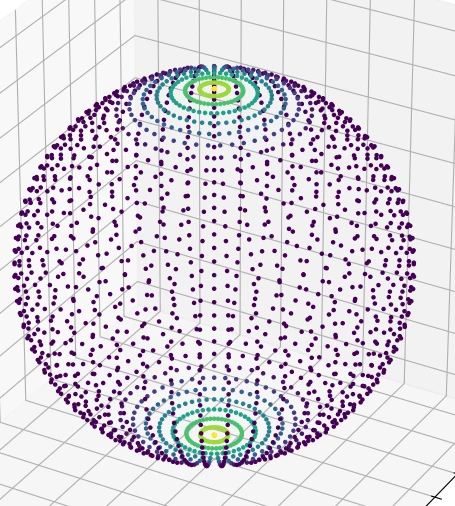
The 2.5° grid drawn on a sphere, coloured by the distance from each point to its nearest neighbour. Points near the equator sit far apart, and the rings at the poles are packed close together.

I weighted each value by the cosine of its latitude $\phi_i$ (in radians). For a score $P_{ij}$ at latitude index $i$ and longitude index $j$, the global value is

$$ \bar{P} = \frac{\sum_{i,j} P_{ij} \cos\phi_i}{\sum_{i,j} \cos\phi_i} $$

The anomaly correlation coefficient compares the forecast anomaly $F' = F - C$ with the observed anomaly $O' = O - C$, where $C$ is the climatological mean:

$$ \mathrm{ACC} = \frac{\sum F' O'}{\sqrt{\sum F'^2 \sum O'^2}} $$

An ACC of 1 means the model predicted the anomaly exactly, 0 means it did no better than forecasting the climatological average, and a negative value means it did worse than that. For $C$ I used the mean of the test data.

Across 2,128 test days, 10,286 grid points, 10 lead times and four scores, each model's comparison covers 875,544,320 measurements.

I did not run IFS or HRES forecasts, so none of the four models is scored against a physics-based baseline. The comparison is between my own models, trained under the same limits.

The four models

Fully connected network

The simplest idea I tried was to feed a whole-globe snapshot into a plain neural network and have it output the weather at a few fixed places for the following days. I chose the grid points nearest Birmingham, London, Paris and Berlin. The input layer has 329,472 values, one layer of 4,096 units follows, then four of 1,024, all with ReLU activations. The output covers 32 parameters at 4 points for 21 days, though I evaluated 10 days of it. Because the forecast points are fixed, latitude weighting would have distorted the scores for this model, so I left it out here.

Convolutional network

The CNN predicts each grid point one day ahead from a 7 × 7 window around it, which spans 17.5° of latitude and longitude, or about 1,942 km north to south. By the Courant-Friedrichs-Lewy (CFL) condition, a window that size over a one-day step can follow a weather front moving at up to 40 km/h. The network has three convolutional layers (32, 64 and 128 filters) followed by three transposed convolutional layers, all with 7 × 7 kernels, ReLU and same padding. It takes 25 values per point and outputs 25 values for the centre point. In tuning, kernel size was the only hyperparameter that made much difference for a model this small.

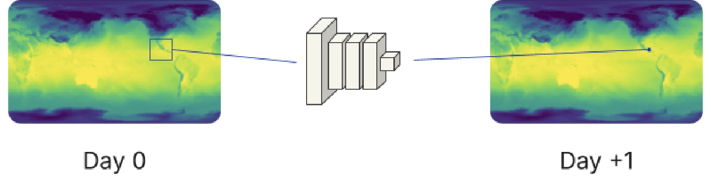
The CNN reads a small window of the day-0 globe and predicts the point at its centre on day +1.

Patch embedding transformer

This follows Pangu-Weather in treating the gridded globe as an image with many colour channels. Pangu embeds the atmosphere with 3D patches and the surface with 2D patches, then merges them. I embedded everything in one 2D patch per location to keep the model simpler.

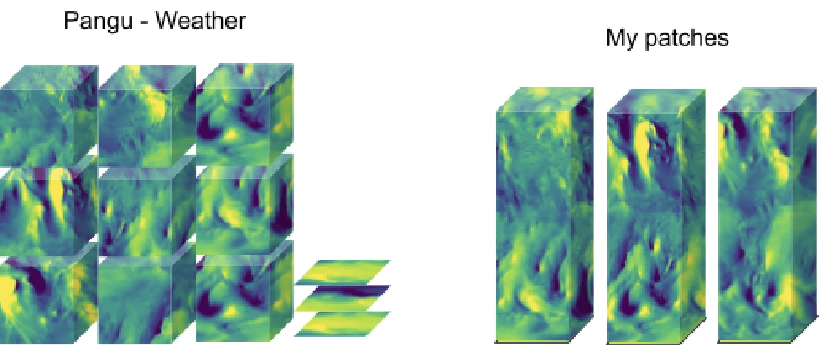
Pangu-Weather's 3D and 2D patches (left) against mine (right), where each patch holds every variable for one latitude and longitude. I wrote this one in PyTorch because I found more material on vision transformers there than for TensorFlow. The one-hour budget forced a choice between 1 × 1 patches with a small model and 2 × 2 patches with an even smaller one. The 1 × 1 version did slightly better, so I kept it: a 32-dimensional embedding and one encoder layer with two attention heads.

Graph transformer

The last model is loosely based on GraphCast. GraphCast encodes the globe onto seven icosahedral meshes (0 to 6 subdivisions) at 0.25°. One of its authors, Ferran Alet, showed in a talk that the multimesh gives only a small gain for pressure variables and does worse on some others. I also found that the finest mesh you can use depends on the input resolution. If the mesh has more points along the equator than the data has longitudes, some mesh points cannot get accurate values. GraphCast has 256 equatorial mesh points sampling 1,439 longitudes. With 143 longitudes, my data only supports three subdivisions.

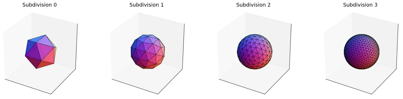
An icosahedron subdivided zero to three times. Three is as fine as 2.5° data allows.

I therefore used a single mesh. That let me feed each output mesh straight back in as the next input, without decoding back to the grid and re-encoding, which adds error. Each mesh point sees itself and its five or six neighbours through a multi-head attention layer (4 heads, 16 key dimensions), followed by layer normalisation, a 64-unit dense layer, dropout of 0.1 and a 25-value output.

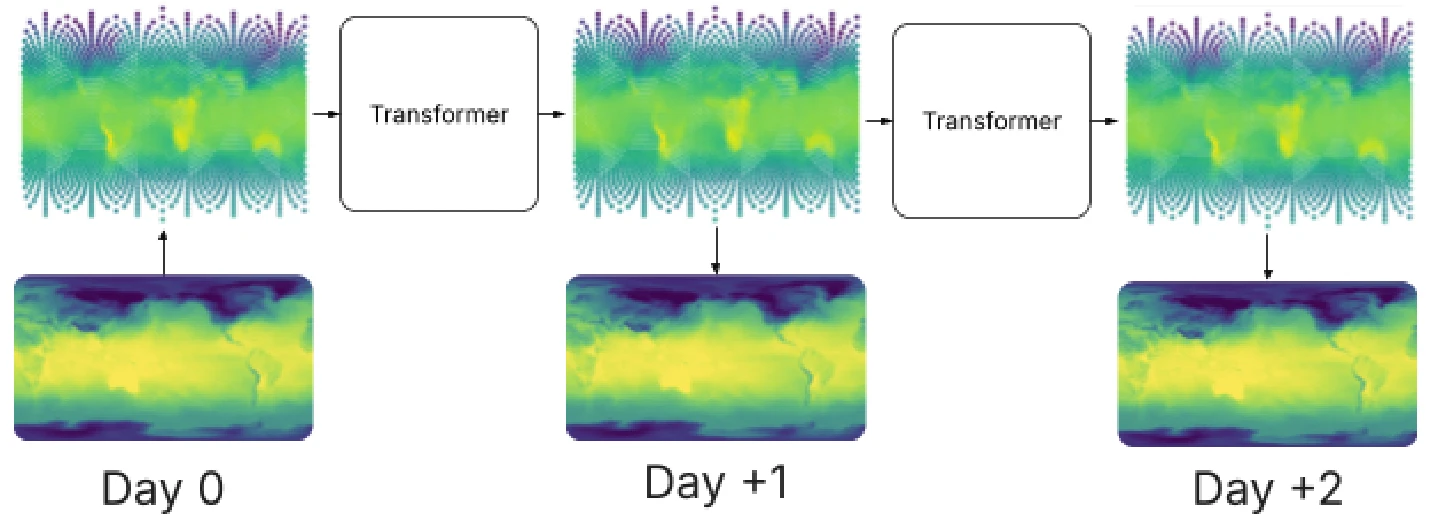
The graph transformer steps from mesh to mesh. Each day's mesh gets decoded to a grid for scoring, but the next step starts from the mesh.

Results

These four charts are the dissertation's results, one per score, for lead times of 1 to 10 days. Lower is better for RMSE and higher is better for ACC.

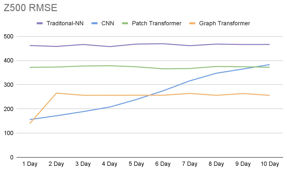
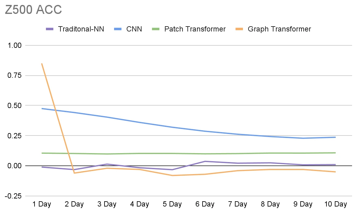
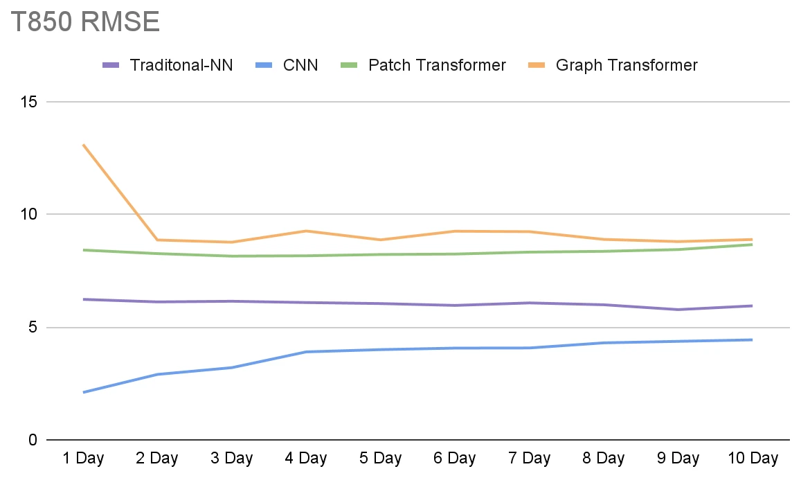
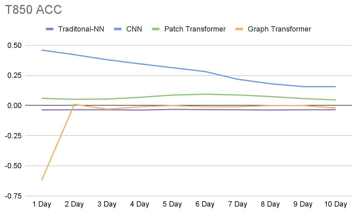
Z500 and T850 scores for all four models. "Traditional-NN" is the fully connected network.

The table sums up the charts.

Model	Z500 RMSE	Z500 ACC	T850 RMSE	T850 ACC
Fully connected	Bad throughout	Poor throughout	Poor throughout	Poor throughout
CNN	Good on day 1, rising slowly to day 10	Reasonable, slow decline	Good, gradually worse	Reasonable, declining
Patch transformer	Bad throughout	Poor throughout	Poor throughout	Poor throughout
Graph transformer	Best on day 1, poor from day 2	Above 0.8 on day 1, negative after	Very poor on day 1, poor from day 2	Extremely poor on day 1, near average after

The fully connected network was barely forecasting. Its Z500 RMSE curve is almost flat because its day-1 predictions were as bad as its day-10 ones. Its ACC went below zero, which points to a bias between training and test data. The test years were warmer: 0.8 °C to 1.2 °C above pre-industrial levels, compared with 0.6 °C to 0.9 °C in the training years. A model that learned the training average would forecast too cold.

The CNN did better than I expected. It had reasonable Z500 and T850 errors for the first few days and kept some skill out to 10 days. When I plotted its 2015 Z500 error by day of year, errors peaked in the middle of the year. The northern hemisphere summer sets the global average temperature, so this fits the same warm bias.

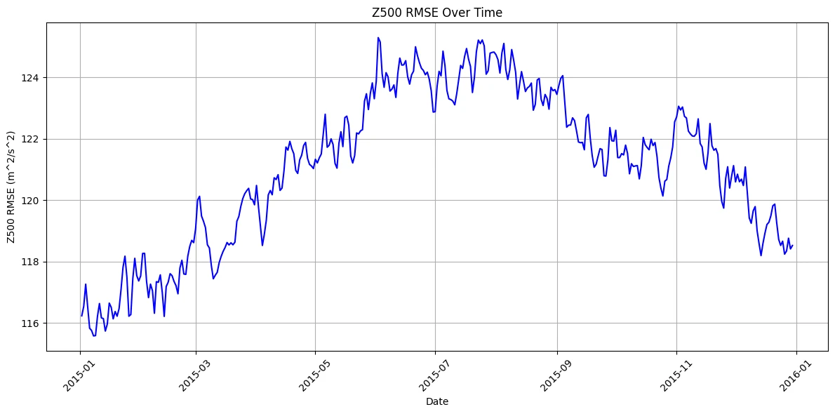
The CNN's Z500 error through 2015, highest in the northern summer.

The patch transformer had high RMSE and low ACC for both variables. It made a visible attempt at Z500, but it started badly and never recovered. At the size I could train in an hour, it underfitted.

The graph transformer gave the most mixed result. Its day-1 Z500 ACC, above 0.8, was the best of any model, roughly the accuracy of a 5-day forecast in 2000. From day 2 every Z500 ACC was negative. T850 went the other way: very poor on day 1, then close to the climatological average. My reading is that turning a 2.5° grid into a coarse mesh smooths out small warm and cold cells, so the temperature field stops matching the rest of the weather. Those errors then feed into the next step and drag the pressure forecast down with them.

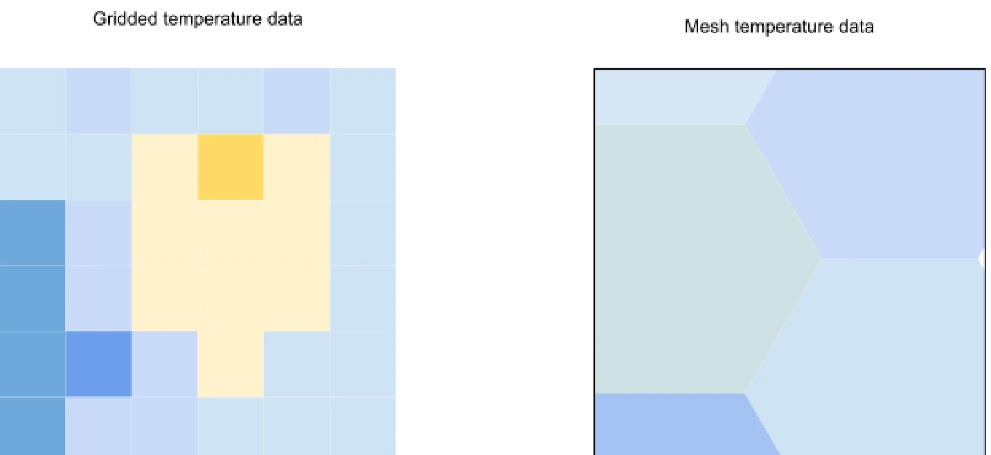
The same patch of temperature on the grid (left) and on a coarse mesh (right). The grid shows a small warm cell that the mesh averages away.

What I concluded

On these results the CNN is the only model worth using. I would still not recommend it for future work. Its main limit is the window size, and a bigger window needs more data than exists. You can get more training samples by shortening the time step, but the CFL condition then shrinks the window. Keep going and each cell only sees its neighbours, which is a numerical model with the physics equations swapped for a network. That would likely perform worse for little saving in compute.

The two transformer models did far worse than their published counterparts, and I expected that during development. The published patch model trained for 700,000 hours, 700,000 times my budget. The mesh for the graph model could not be any finer than the 2.5° data allowed.

The graph model predicted low-frequency features like pressure well from good inputs, even while its temperature and wind forecasts were poor. I recommended that future work build on a mesh, with three changes:

• Build the mesh directly from data assimilation rather than encoding it from a gridded dataset, so it can reach the resolution that high-frequency weather needs.
• Use larger transformers. They cost more to train and run than mine, but still far less than numerical models.
• Match the area each point looks at to the time step using the CFL condition, and use long steps of 12 or 24 hours, since longer steps have given better accuracy at medium range.

For the graph model in particular, I would fine-tune at the end of training on its own outputs as inputs. It should then learn to trust the pressure variables it predicts well over the atmospheric ones it predicts badly. A finer mesh would also help.

Limitations

This comparison was small. Each model had one hour on one GPU, used 2.5° data, and took daily steps. That setup was deliberate, since it gave each architecture equal footing, but the results may not show how these designs perform at scale. The transformers suffered most. I also did not compare against an operational forecast such as HRES, so the results rank the architectures against each other and give no measure of their skill next to a physics-based model.

A related video shows a smaller CNN I trained running: youtu.be/wHGRG7PzSQc.